Iterative Riemann Solver for Interface Interaction in Compressible Multiphase Flows

Rishabh Datta is a 4th Year Mechanical Engineering student at Georgia Tech, Atlanta. Rishabh is interested in Energy and Fluid Systems, CFD and renewable technology. For more projects, click here.

Interface Interaction in Multiphase Flows

Introduction

Multiphase flows of compressible fluids can be simulated using different numerical methods. In the interface-ghost fluid method introduced by Hu, 2004, multiphase flows are simulated by solving the single phase equations within each fluid, and solving the real and ghost fluid interactions at the interface. The interface movement is captured using a level-set function, where the zero level-set marks the position of the interface in a multi-fluid system. The interaction at the interface constitutes a two-material Riemann problem. In this report, the two-material Riemann problem at the interface is solved for two compressible, inviscid and immiscible fluids. The effect of capillary forces and the presence of large discontinuities in impedances of the materials is also considered. The results are them compared with standard test cases, whose results have been obtained from an exact Riemann solver.

Interface Interaction

Compressible inviscid flow in 2D can be described using the Euler equations as follows:

\begin{bmatrix} \rho \\ \rho u \\\rho v \\ E \end{bmatrix} _{t} + \begin{bmatrix} \rho u \\ \rho u^{2} + p \\ \rho uv \\ (E+p)u \end{bmatrix} _{x} + \begin{bmatrix} \rho v \\ \rho uv \\ \rho v^{2} +p \\ (E+p)v \end{bmatrix} _{y} = 0

where \rho is the density, u and v are the components of velocity and the x and y directions respectively, p is the pressure, and $$E = \rho e + 1/2 \rho u^2$$ is the total energy density.

The method of characteristics was used to solve the two material Riemann problem at the interface. In the presence of capillary forces, a pressure drop is experienced at the interface between the region near the interface in the left fluid, and that in the right fluid. The pressures of the two fluids near the interface change to $p_{I,l}$ and $p_{I,r}$ , where:

p_{l} - p_{r} = \sigma k

where $\sigma$ is the coefficient of surface tension, and k is the curvature.

For isentropic interface intercation, the velocity at the interface $u_{I}$ can be represented as:

u_{I} = u_{l} - \int_ {p_{l}}^{p_{I,l}} \frac {dp}{ \rho_ {l,s}c_{l,s}}

u_{I} = u_{r} + \int_ {p_{r}}^{p_{I,r}} \frac {dp}{ \rho_ {r,s}c_{r,s}}

The set of equations need to be closed using an appropriate equation-of-state (EOS). The Stiffened Gas EOS, which was used, can be represented as follows:

p = (\gamma -1)\rho e - B

Isentropic EOS can be written as follows:

These equations can be rewritten as:

\frac{f(p)}{ \rho^{ \gamma}} = constant

where $f(p) = p$ for an ideal gas, and $f(p) = p + B$ for a stiffened gas. \\

where $\gamma$ is the specific heat ratio and B is the reference pressure.

These equations can be rewritten as:

u_{I} = u_{l} - \frac{2c_l}{\gamma_l -1}\left[\left(\frac{f_l(p_{I,l})}{f_l(p_l)}\right)^{(\gamma_l -1)/2\gamma_l}-1\right]

u_{I} = u_{r} + \frac{2c_r}{\gamma_r -1}\left[\left(\frac{f_r(p_{I,r})}{f_r(p_r)}\right)^{(\gamma_r -1)/2\gamma_r}-1\right]

p_{I,l} - p_{I,r} = \sigma k

The above system of equations can then be solved numerically with an appropriate iterative root-finding algorithm. The Newton-Rhapson Method was used to determine the pressures and velocity at the interface.

The Sod Shock Tube Problem

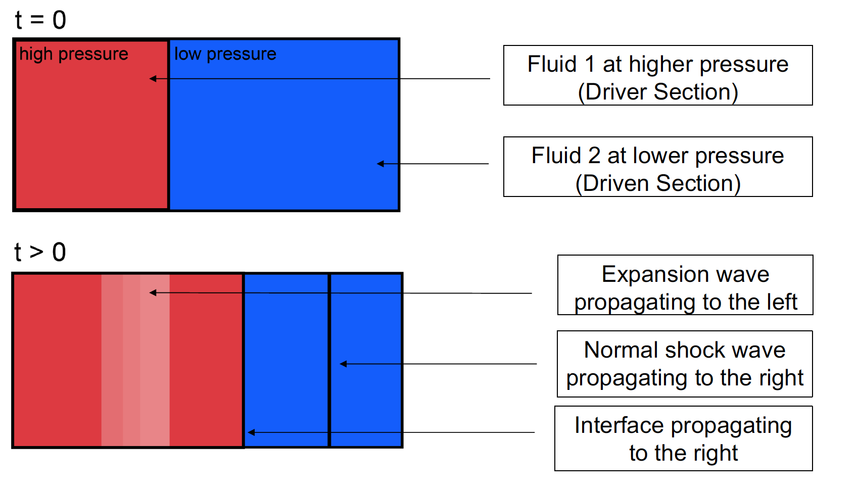
Shocktube configurations at t = 0 and t > 0

The Sod shock tube problem is an air-helium shock tube which can be initialized with the following conditions:

(\rho, u, p, \gamma) = (1.0, 0.0, 1.0, 1.4), (x \leq 0.5)

(\rho, u, p, \gamma) = (0.125, 0, 0.1, 1.667) , (x > 0.5)

The simple shock tube configuration is shown above. The shock tube problem was solved numerically and compared with the results from the exact Riemann solver at t = 0.2s. The method is able to correctly capture the shock strength and speed, as well as the location of the contact interface. The method introduces errors, especially near the contact interface, and to some degree, in the rarefaction wave region of the shock tube. However, the magnitude of the error can be observed to decrease at higher resolutions.

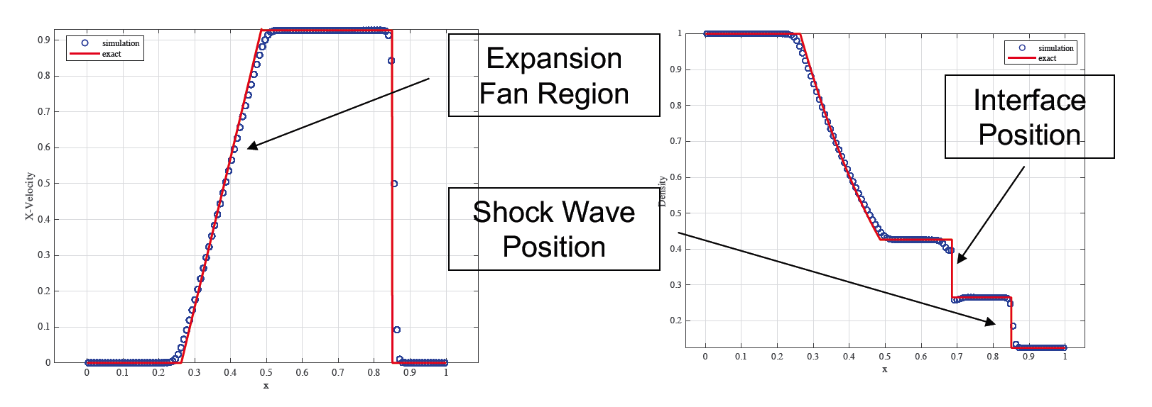
Variation of velocity and density along Shock Tube at t = 0.2s

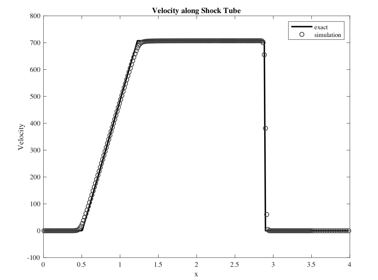
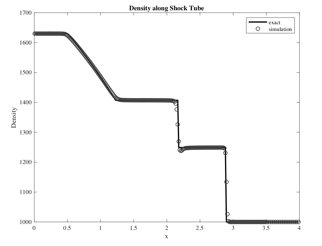
Hydrodynamic Shock Tube Problem

The hydrodynamic shock tube problem was be initialized with the following conditions:

(\rho, u, p, \gamma) = (1630.0, 0.0, 7.81e9, 7.15) , (x \leq 2)

(\rho, u, p, \gamma) = (0.125, 0, 0.1, 1.667) , (x > 2)

The shock tube problem was solved numerically and compared with the results from the exact Riemann solver at t = 0.00025 s. The Stiffened Gas EOS of state was used, with a reference pressure $B = 3.309e8$ . The results from the simulation were found to be in good agreement with the exact solution. Again, the numerical method seems to introduce errors near the contact discontinuity, but the magnitude of the error can be reduced by running the simulation at higher resolutions.