Computing Cut Cell Apertures, Interface Area and Volume Fraction

Introduction

In multiphase flows, the interface between two fluids can be expressed using a level set function, which is a signed scalar function \Phi(x,t) such that | \triangledown \Phi | = 1. One of the fluids can be defined as the positive phase, i.e. \Phi (x,t) > 0 , and the other is defined as the negative phase i.e. \Phi (x,t) < 0. The interface between the two fluids \Gammais represented by the zero level set, \Phi (x,t) = 0. A cut cell can be defined as a cell that contains the local interface. In this report, we assume a sharp interface, i.e. each cell is cut by the interface only once. The volume fraction of the cell can be determined from the cell face apertures, the interface area \Delta \Gamma and the level set values at the cell center.

Delaunay Triangulation

The interface area \Delta \Gamma and the cell face apertures can be calculated using Delaunay triangulation, by diving the total area into a set of triangles. The sum of the areas of each triangle is then the total enclosed area. In Delaunay triangulation, individual triangles are formed such that they conform with the following criteria:

• The triangles are empty. No other vertices or edges can be contained in an individual triangle.
• The circumcircle of each triangle is empty. No other vertices belonging to other elements of the set can be contained in the circumcircle.

To check if a triangle is empty, it is necessary to determine if a potential edge of a new triangle intersects with edges of existing triangles. In 3-D, the point of intersection P(x,y,z) of two lines AB and CD (representing the potential edge and an existing edge) can be determined by solving the parametric line equations in R^{3}.

Given that AB and CD are not skew or parallel, the two edges intersect if P lies along both edges.

To check if the circumcircle of $\Delta ABC$ is empty, it is necessary to determine the circumcenter $Q(x_{c},y_{c},z_{c})$ of $\Delta ABC$ . The circumcenter is the point which is equidistant from vertices A, B and C. In R^{3}, the circumcenter of a triangleis given by the equation below. The radius r of the circumcircle can then be determined form the Euclidian norm of the vector connecting the center $Q$ to one of the triangle vertices. A point P lies inside the circumcircle if the Euclidian norm of $\overrightarrow{PQ}$. is less than the radius of the circumcircle. The circumcircle is considered not empty in this case.

Level Set Values at Cell Corners and Determining Cut Points

The level set values at cell corners can be determined from the arithmetic mean of the level set values at the cell centers of the surrounding cells. From the level set values at cell corners, the position of the cut points in a cut cell can be determined by linear interpolation. For a given edge enclosed by corners A and B, the level set values at $A(x_{1},y_{1},z_{1})$ and $B(x_{2},y_{2},z_{2})$ can be represented by $\Phi_{1} $ and $\Phi_{2} $ respectively. If $ \Phi_{1}\Phi_{2} < 0 $ , then a cut point lies on the given edge. The coordinates of the cut point are given by:

Cell Volume Fraction

The volume fraction and cell face apertures are computed with respect to the positive fluid. From the cell face apertures and level set value at cell center $\Phi_{c}$ , the volume fraction \alpha can be calculated as:

$A^{11}$ and $A^{12}$ are the cell face apertures on the west and east faces respectively, $A^{21}$ and $A^{22}$ are the cell face apertures on the south and north faces respectively, and $A^{31}$ and $A^{32}$ are the cell face apertures on the bottom and top faces respectively.

Methodology

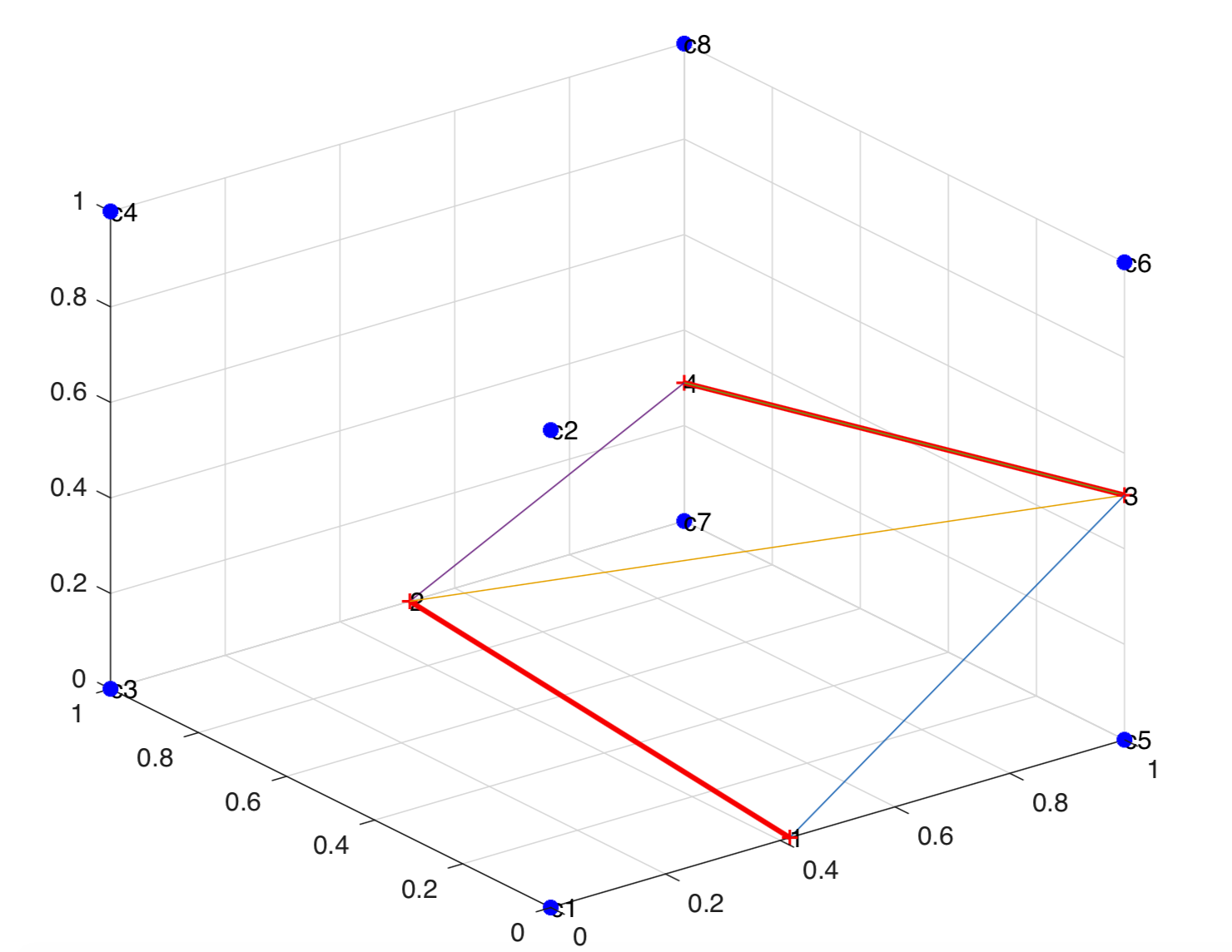
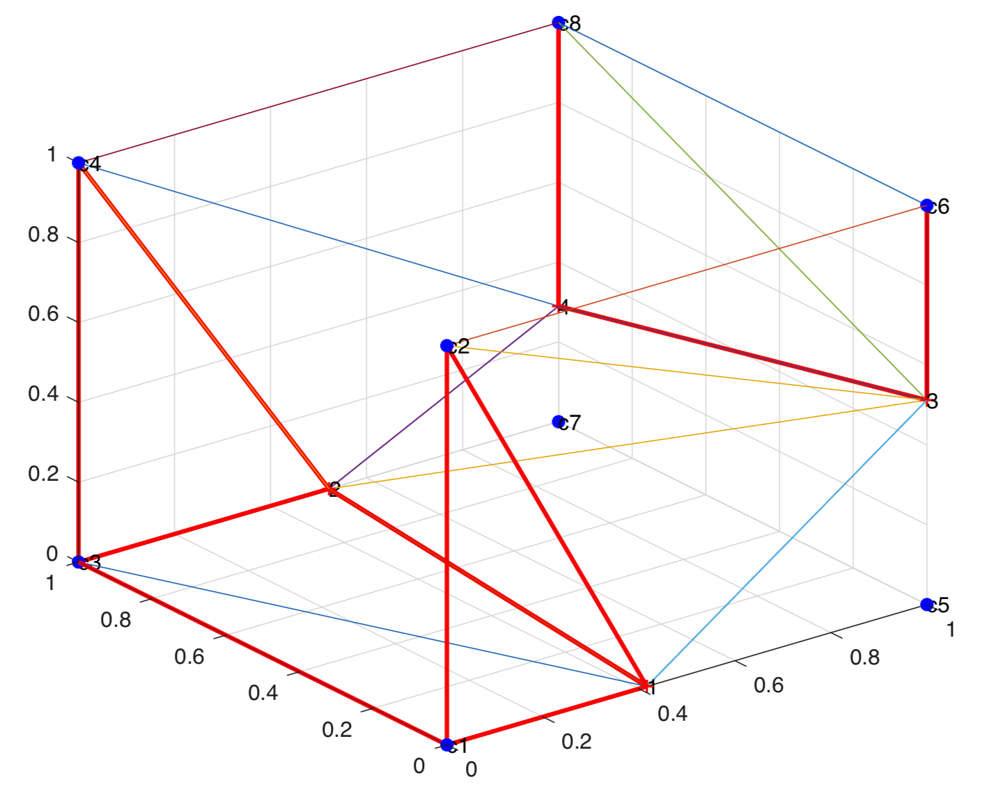
The cut points were first determined for the given cut cell from the level set values at the cell corners. The cut points were then triangulated to determine the local interface area . The cut points are shown in the figure below.

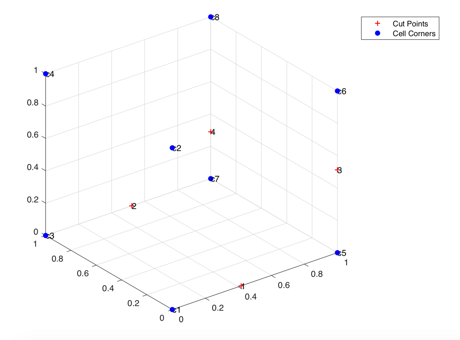
Cut points are determined from the level set values at cell corners

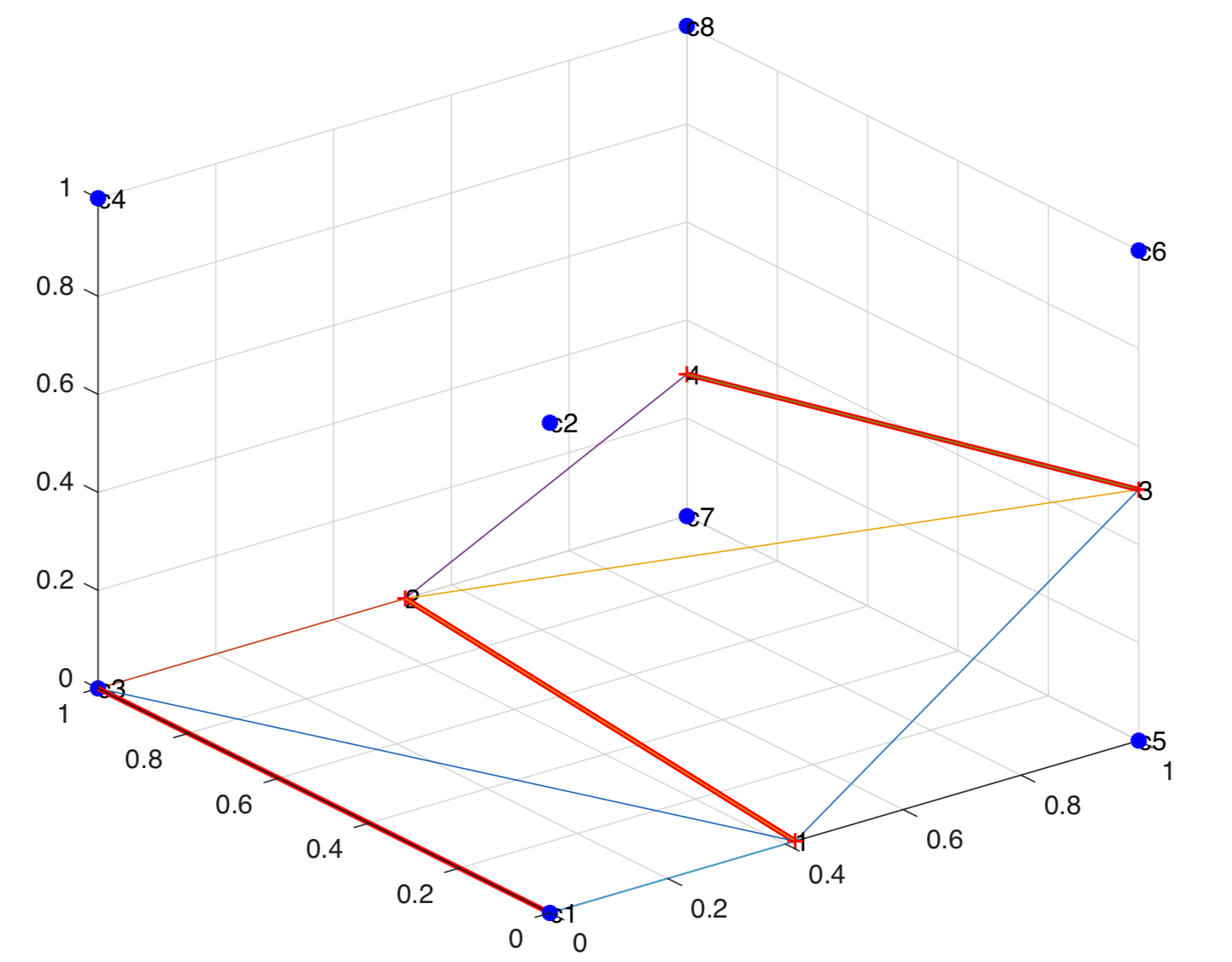
To triangulate a set of co-planar points in $R^{3}$, the Divide and Conquer algorithm was used. The points to be triangulated were first sorted lexicologically, i.e. they were first sorted by x-coordinate, then by y-coordinate and then by z-coordinate. For a sharp interface, the interface cuts the cell at at most 4 points. These points are then divided into two subsets. Subset 1 contains the first two points after lexicological sorting, and the Subset 2 contains the remaining points. In each subset, the points are then connected separately. The two subsets are then merged. In order to merge the subsets, the low tangent is first identified. The low tangent connects the ``lowest'' points in each subset. The lowest points can be identified by sorting the points in each subset clockwise with respect to the plane normal, then starting form the first point in Subset 1, and moving anti-clockwise to the next point until the next point lies in Subset 2. Similarly, the lowest point in Subset 2 is identified by moving clockwise form the last point in Subset 2, until the next point lies in Subset 1. Given the geometry of the cut points, the low tangent can be determined by connecting the first point in Subset 1 to the point in Subset 2 which lies closest to it.

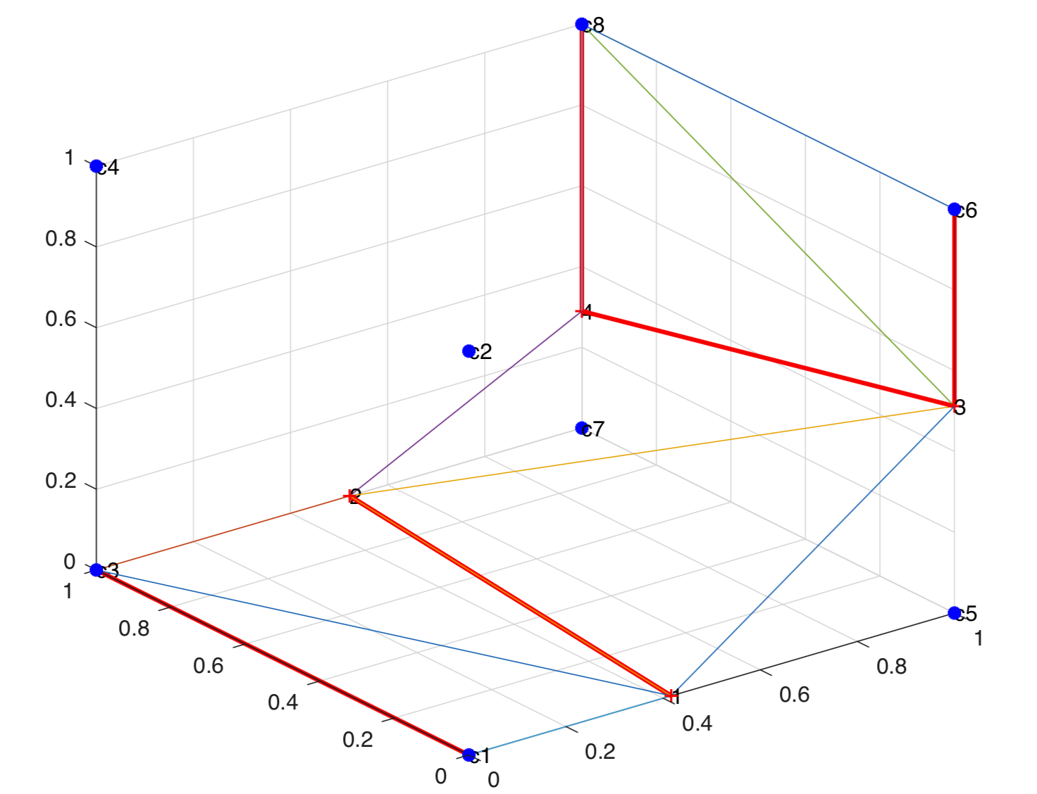
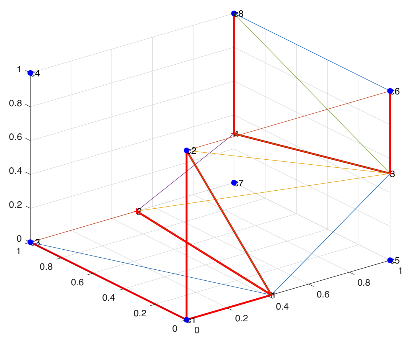
On forming the low tangent, it is necessary to identify the third vertex to form a Delaunay triangle. Of the two possible candidates for the third vertex, the candidate is chosen for which the new triangle and its circumcenter are empty, thus fulfilling the Delaunay criterion. The last point is then connected to the existing edge to create another triangle. The sum of the areas of each individual triangle is used to determine the interface area.

For a given face, the maximum number of points to triangulate is 5 due to the geometry of the cut face. The aforementioned Divide and Conquer algorithm can be used for this purpose. In the case of five points, Subset 1 contains the first 3 points in lexicological order, while Subset 2 contains the remaining points. The points on the edge of the triangle in Subset 1 which should be used to form the low tangent can be determined by identifying the edge for which a potential low tangent does no intersect with any existing edges. The triangulation can then be continued as mention before.

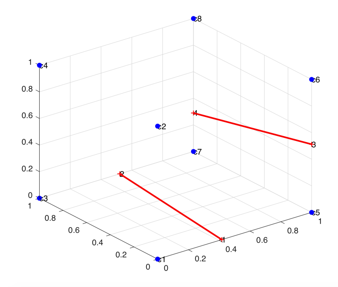
The points in each subset are connected separately

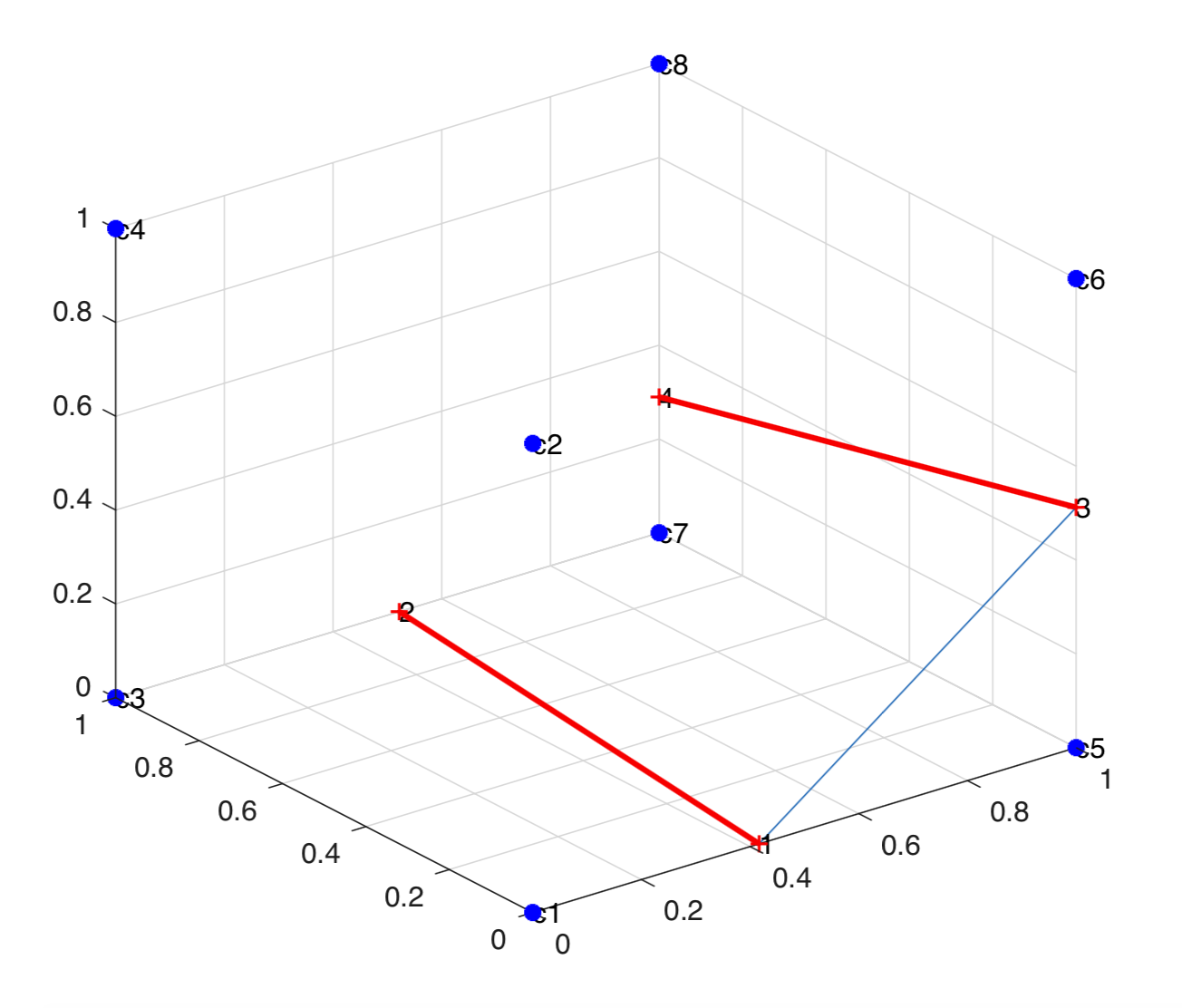
The low tangent is formed

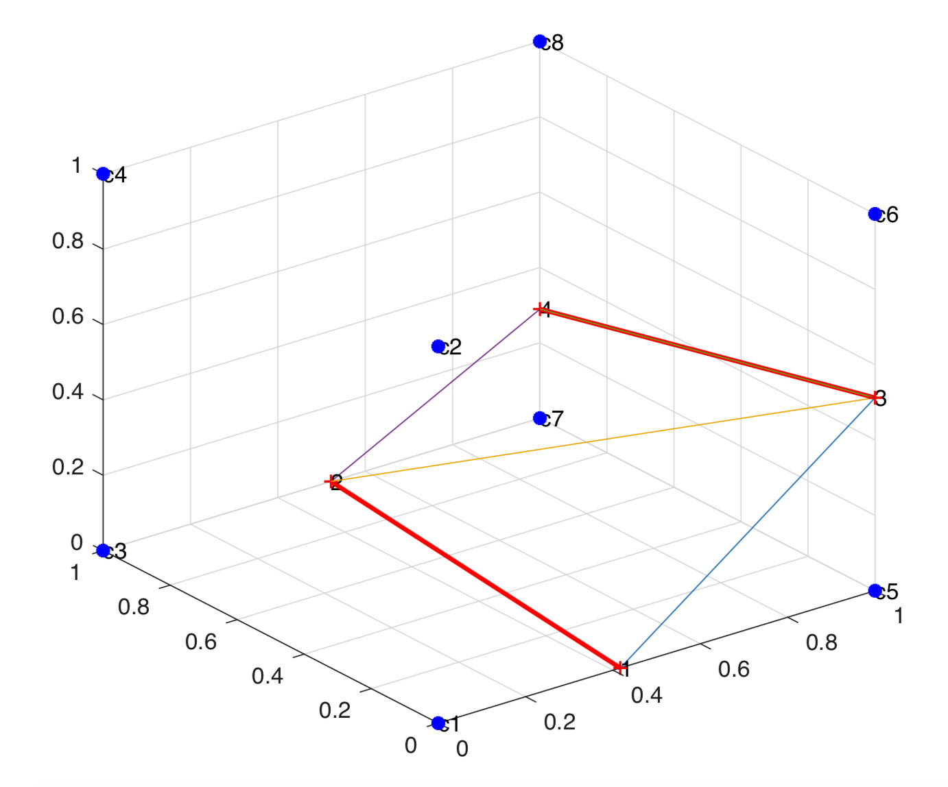
The last point is connected to complete the triangulation

The cell face apertures are determined using a similar approach. First, the cell corners are sorted lexicologically. The faces are then checked to see if they contain only the positive fluid , i.e. the number of face corners with positive level set value is 4. For a face with only positive fluid, the cell face aperture is 1. For faces with the negative fluid, the cut points which lie in the face are determined. For a given cut point P, it lies on the given face if and only if the dot product of the vector connecting a point Q on the face to the cut point and the normal to the plane is zero.

If the number of cut points on the face is zero, the cell face aperture is 0. If the number of cut points is non-zero, then the corners of the face with positive level set values is determined. These points are then triangulated to determine the area occupied by the positive fluid. The ratio of this area to the total area of the face is the cell face aperture for the given face. Triangulation to determine different apertures is shown below.

Triangulated Interface

Bottom face is triangulated to get A31

Bottom face is triangulated to get A12

South face is triangulated to get A21

North face is triangulated to get A22

Implementation

The method presented was used to determine the cell volume fraction and cell face apertures. For greater accuracy, a given cell was refined once, and the cell volume fraction was determined from the arithmetic mean of the cell volume fractions of each sub cell. In 3D, each cell was divided into 8 subcells, and the sub cell volume fraction of each individual cell was first computed. Similarly in 2D, each cell was divided into 4 sub cells, and in 1D, each cell was divided into 2 sub cells. Each parent cell was also assumed to have a cell size of 2, with the cell center located at (1,1,1). Each sub cell center was then determined by iteratively travelling a distance of $(0.25 \times \textrm{cell size)}$ in the $\pm x, $\pm y and $\pm z directions from the cell center. The cell corners of a given sub cell were then determined similarly, by moving a distance of $(0.5 \times \textrm{sub cell size)}$ in the $\pm x, $\pm y and $\pm z directions from the sub cell center.